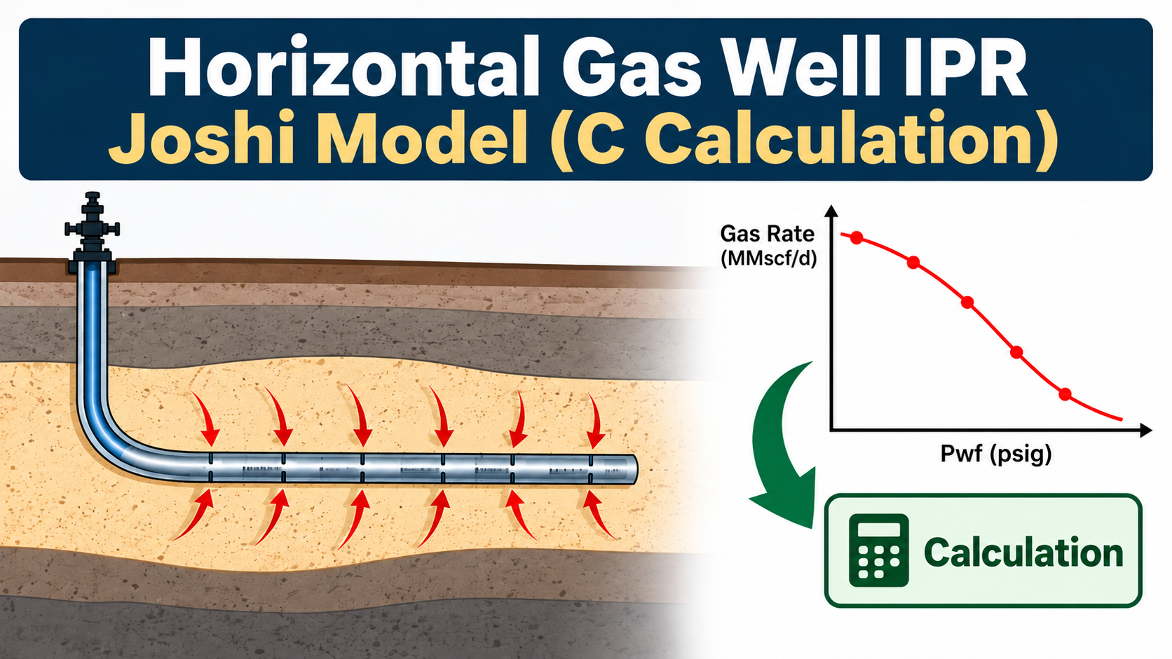
Horizontal Gas Well IPR: Using the Joshi Model to Estimate a Representative PROSPER C

Horizontal Gas Well IPR: Using the Joshi Model to Estimate a Representative PROSPER C

Horizontal gas wells can deliver significantly different inflow performance compared with conventional vertical wells. When a development horizontal well must be calibrated from an existing vertical DST, simply transferring the DST deliverability coefficient C is generally not sufficient.

A more practical workflow is to use the Joshi horizontal-well productivity model to generate a physically based horizontal-well inflow performance relationship, then fit a representative C for use in PROSPER while retaining the tested gas deliverability exponent n.

Petrotopic Calculator:
Horizontal Gas Well — Joshi C Calculator | Petrotopic

1. Why is horizontal gas-well IPR different?

A vertical well and a horizontal well do not expose the reservoir to flow in the same way.

A vertical DST may represent flow through only a limited perforated interval, while a horizontal open-hole well can contact a much larger section of the reservoir.

Important parameters include:

Horizontal permeability, kh
Vertical permeability, kv
Reservoir thickness, h
Horizontal well length, L
Drainage radius, re
Wellbore radius, rw
Horizontal-well skin, S
Gas viscosity, μg
Gas compressibility factor, Z
Reservoir pressure, Pr
Flowing bottomhole pressure, Pwf

Therefore, the development-well IPR should ideally be calculated using the actual horizontal-well geometry rather than simply copying the vertical DST C value.

2. Recommended workflow

A practical workflow is:

Vertical DST → PVT → Gas pseudopressure → DST kh → Partial-penetration assessment → Development kh → Joshi horizontal IPR → PROSPER C

The key idea is to separate the DST interpretation from the development horizontal-well model.

This allows the engineer to change development permeability or horizontal-well skin without modifying the original DST interpretation.

3. Permeability anisotropy

The Joshi model accounts for different horizontal and vertical permeability.

The anisotropy factor is:



where:

kh = horizontal permeability
kv = vertical permeability
β = permeability anisotropy factor

For example, if:

kv / kh = 0.1

then:

kh / kv = 10

and:

β = √10 = 3.162

A larger difference between horizontal and vertical permeability changes the effective flow resistance around the horizontal well.

4. Why gas pseudopressure should be used

For gas wells, viscosity and compressibility factor change with pressure.

Instead of assuming that gas behaves with constant μg and Z, the gas pseudopressure can be calculated from the PVT data.

The gas pseudopressure is:



where:

p = absolute pressure
μg = gas viscosity
Z = gas compressibility factor
m(p) = gas pseudopressure

The pressure must be absolute pressure, not gauge pressure.

Therefore:

pabsolute = pgauge + 14.7 psi

approximately at standard atmospheric pressure.

5. Numerical calculation of pseudopressure

In a spreadsheet, the integral can be calculated using the trapezoidal method.

For two consecutive PVT pressure points:



Then:



The required pseudopressure difference is:



This method has an important practical advantage: the calculation can be audited directly from the PVT table.

6. Interpolating pseudopressure

The reservoir pressure or flowing pressure will often not exactly match one of the PVT pressure points.

For example, the PVT table might contain:

2000 psig
2300 psig
2800 psig

while the required pressure is 2300 psig.

If the pressure falls between two PVT points, linearly interpolate the accumulated pseudopressure.

This gives:

m(Pr)

and:

m(Pwf)

Then:


7. Estimating apparent DST permeability

The vertical DST can first be interpreted using a conventional radial-flow model.

A simplified gas pseudopressure relationship can be represented as:



where:

q = gas rate
kh = effective permeability
h = flowing reservoir thickness
Δm = gas pseudopressure difference
TR = reservoir temperature in Rankine
D = flow-resistance term

For a simple vertical radial-flow reference case:



where:

re = drainage radius
rw = wellbore radius

This provides an apparent DST permeability.

It should not automatically be assumed to be the true development-well kh.

8. Partial penetration of the DST

Partial penetration can be important when the DST tests only part of the reservoir.

For example:

Total reservoir thickness = 75 m

while:

DST tested interval = 10 m

The DST therefore does not necessarily represent full-thickness reservoir inflow.

An Odeh-type partial-penetration correction can be used to assess this effect.

One form of the correlation is:



where:

ht = total reservoir thickness
hp = tested/perforated interval
kH = horizontal permeability
kV = vertical permeability
rwc = corrected wellbore radius

The correlation should be applied consistently with the units and assumptions of the source formulation.

9. Do not double-count partial penetration

This is an important engineering point.

There are two separate concepts:

DST interpretation

The partial-penetration correction can be used to understand what the DST permeability might represent.

Development horizontal well

The horizontal well has its own geometry and potentially its own skin.

Therefore:

DST partial-penetration correction ≠ horizontal-well skin

If the DST permeability has already been corrected for partial penetration, that correction should not simply be added again as horizontal-well skin.

10. Development-well kh should remain editable

For a development horizontal well, it is useful to keep kh as a direct engineering input.

For example:

Case kh
Low case User input
Base case User input
High case User input

This is particularly useful in heterogeneous carbonate reservoirs where permeability can vary significantly.

A DST-derived permeability can therefore be retained as a reference or sensitivity case, rather than automatically forcing the development well to use exactly the same value.

11. Joshi horizontal-well model

The Joshi model accounts for the geometry of the horizontal well and the reservoir.

The horizontal-well effective drainage parameter can be calculated from:



where:

L = horizontal well length
reh = effective drainage radius

The effective drainage radius can be represented by:



where:

A = drainage area

The Joshi flow-resistance term can then be written as:



This term represents the geometric resistance associated with the horizontal well.

12. Horizontal gas-well inflow using pseudopressure

The gas inflow can then be represented in the form:



where:

qg = gas production rate
kh = horizontal permeability
h = reservoir thickness
Δm = gas pseudopressure difference
TR = reservoir temperature in Rankine
DJoshi = Joshi flow resistance
S = horizontal-well skin

The exact constant and unit system must remain consistent with the units used in the implementation.

13. Why horizontal-well skin should be an independent input

Skin is not necessarily a fixed reservoir property.

For an open-hole horizontal well, the effective skin may depend on:

Completion condition
Formation damage
Cleanup
Near-wellbore permeability
Completion quality
Open-hole exposure
Reservoir heterogeneity

Therefore, it is useful to allow the user to test several skin values.

For example:

S = −4

S = −2

S = 0

S = +1

S = +2

This provides a practical sensitivity range rather than assuming that one skin value is universally correct.

14. Generate the complete horizontal IPR

One of the most important aspects of this methodology is that the horizontal-well flowing pressure does not need to be assumed in advance.

Instead, calculate the Joshi rate at multiple flowing pressures.

For example:

Pwf Joshi q
High Pwf Low
↓ ↓
Medium Pwf Medium
↓ ↓
Low Pwf High

This produces a complete horizontal-well IPR.

The result is more useful than calculating only one production rate at one assumed flowing pressure.

15. Converting the Joshi IPR to PROSPER C

PROSPER can represent gas deliverability using a C–n relationship.

In a common form:



Depending on the PROSPER setup, the exact pressure convention and units should be checked before entering the final coefficient.

The important point is that n can be retained from the DST.

For example:



Then the horizontal Joshi IPR can be used to determine a representative:



where:



for the corresponding pressure convention.

16. Why fit C over the complete IPR?

A common temptation is to calculate C from one selected flowing pressure.

For example:

"At 1500 psi flowing pressure, the horizontal well produces X MMscf/d, therefore C = Y."

This can be misleading because C then becomes strongly dependent on the selected Pwf.

A better approach is:

1. Generate the complete Joshi IPR.

2. Calculate C at multiple Pwf values.

3. Examine the resulting C values.

4. Fit a representative C while keeping n fixed.

This produces a C that represents the overall horizontal-well inflow behaviour rather than one arbitrary operating point.

17. Example engineering data

Consider a development case with:

Parameter Example
Reservoir thickness 75 m
Horizontal well length 548 m
Drainage radius 500 m
Wellbore radius 0.122 m
kv/kh 0.1
Horizontal permeability 50 mD
Horizontal skin 0
Reservoir pressure 2300 psig
DST n 0.89202

The anisotropy factor is:



The actual values should be replaced with the engineer's reservoir and well-specific inputs.

18. DST permeability versus development permeability

It is useful to keep these concepts separate.

DST apparent permeability

This comes directly from interpreting the DST.

It reflects the tested interval and the flow geometry of the DST.

DST corrected permeability

A partial-penetration correction may be applied to understand a full-thickness equivalent permeability.

Development kh

This is the permeability selected for the horizontal development-well model.

It may be:

Equal to the geological model value
Calibrated from DST interpretation
Calibrated against nearby wells
Used as a sensitivity parameter

There is no requirement that all three values be identical.

19. What the Petrotopic calculator provides

The Petrotopic calculator brings these calculations into one workflow.

Input

The user can enter:

kh
kv/kh
Reservoir thickness
Horizontal well length
Drainage radius
Wellbore radius
Skin
Reservoir pressure
Reference flowing pressure
Gas deliverability exponent n
Temperature
Gas PVT data
Calculation

The calculator then:

Processes the PVT table.
Converts pressure to absolute pressure where required.
Calculates gas pseudopressure.
Interpolates m(Pr) and m(Pwf).
Calculates Δm.
Calculates the Joshi geometry.
Calculates horizontal-well inflow.
Generates the IPR.
Determines the representative C using the specified n.
20. Why this approach is useful for PROSPER

A reservoir engineer may have a detailed horizontal-well model but ultimately need a practical inflow relationship for a nodal-analysis model.

The Joshi calculation provides the physical basis.

PROSPER then receives a simplified deliverability representation:

Joshi physical model → representative C–n model

This allows the horizontal-well inflow to be incorporated into a larger production-system model while retaining a clear link back to the reservoir and well assumptions.

21. Important limitations

The Joshi model is an analytical productivity model.

It should not be interpreted as a complete reservoir simulation.

For example, the basic analytical model does not automatically reproduce:

Complex natural fractures
Explicit dual-porosity behaviour
Explicit dual-permeability behaviour
Strong reservoir heterogeneity
Complex pressure-dependent permeability
Transient multiphase effects
Detailed completion inflow distribution
Water or condensate effects

Therefore, the calculated C should be considered a representative engineering coefficient, not a universal reservoir constant.

22. Recommended sensitivity analysis

For development planning, I recommend testing at least:

Permeability sensitivity

Low kh → Base kh → High kh

Skin sensitivity

Negative skin → Zero skin → Positive skin

Reservoir pressure sensitivity

Low Pr → Base Pr → High Pr

Horizontal length sensitivity

Shorter L → Base L → Longer L

This allows the engineer to understand which assumptions have the greatest impact on the resulting C.

23. Practical workflow summary

The complete workflow can be summarized as:

Step 1 — DST

Obtain:

qDST, Pr,DST, Pwf,DST, nDST

↓

Step 2 — PVT

Prepare:

Pressure, Z, μg

↓

Step 3 — Pseudopressure

Calculate:

m(Pr), m(Pwf), Δm

↓

Step 4 — DST permeability

Calculate apparent DST kh.

↓

Step 5 — Partial penetration

Assess the impact of the tested interval.

↓

Step 6 — Development kh

Select an appropriate development-well kh.

↓

Step 7 — Horizontal geometry

Enter:

L, h, re, rw, kv/kh

↓

Step 8 — Horizontal skin

Apply the selected development-well skin.

↓

Step 9 — Joshi IPR

Generate q for multiple Pwf values.

↓

Step 10 — PROSPER C

Keep:

n = nDST

and fit:

C = representative horizontal-well deliverability coefficient

24. Final takeaway

The objective is not simply to calculate a new C from a single horizontal-well pressure point.

The more useful engineering approach is:

Use the DST to establish the gas deliverability behaviour and reservoir reference, use PVT pseudopressure to properly account for gas properties, use the Joshi model to represent the horizontal-well geometry, generate the complete horizontal IPR, and finally fit a representative PROSPER C while keeping n consistent with the DST.

This provides a transparent connection between the tested vertical well, the horizontal development well, and the PROSPER inflow model.

Try the calculator

Horizontal Gas Well — Joshi C Calculator

Open the calculator on Petrotopic

The calculator is intended to make the workflow practical by allowing the engineer to change kh, kv/kh, horizontal length, reservoir thickness, drainage radius, skin, reservoir pressure and PVT data and immediately see the effect on the calculated horizontal-well inflow and representative C.

Engineering note

The equations above are presented in simplified, web-friendly form for practical engineering use. Always verify the unit system, pressure convention, correlation applicability and PROSPER input convention before using a calculated C in an actual well model.